Binarized Random Projected SIFT descriptors
In this project, we investigate how robust and distinctive SIFT descriptors are, when they are projected and binarized using so called Random Projections and a simple sign function.
The main goal of this work is to provide an analysis of the statistical properties, and thus the discriminative power, of binarized projected SIFT descriptors. We will primarily investigate the binarized projected SIFT fingerprint statistics on real image datasets, and the statistics of the fingerprints under various distortions.
The dataset used, is the Airplane subset from the Caltech 101 dataset.
Architecture
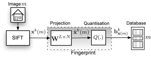
Random Projections
Implementation
Random projections are implemented in the function m_pr.m. Example usage is W = m_rp(L, N) where L is the Number of rows of W, or input dimension and N is the Number of columns of W, or the number of dimensions to project to.
Testing
There are three basic tests
- Testing intra image descriptor statistics.
- Testing channel distortion statistics.
- Testing inter image descriptor statistics.
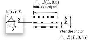
Intra Image descriptor statistics
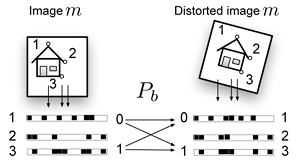
Channel distortions
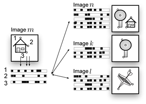
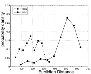
Inter image descriptor statistics
Results
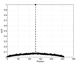
Correlations within individual descriptors before and after projection
Below are the average normalized Autocorrelation function values of all descriptors before and after projection. This shows the correlation within each individual binarized projected descriptor, which after projection is virtually zero. These descriptors behave as if generated by \(\mathcal{B}(L, 0.5)\).
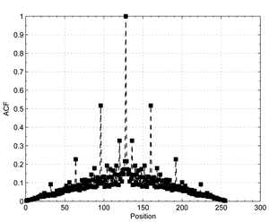
Some residual correlation is still present between all descriptor vectors. This follows from the fact that Random Projections are fast, but not optimal. Also, as SIFT descriptors are designed for robustness, equal image patches will result in similar SIFT descriptors in the dataset. Correlation between binarized projected SIFT vectors can be modelled as \(\mathcal{B}(L, 0.3)\).
Channel distortions
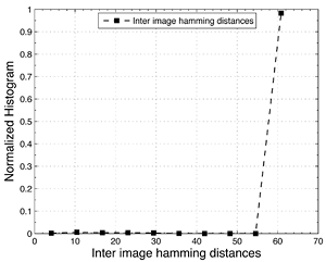
If we look at the statistics of binarized projected descriptors when matching identical but distorted images against eachother, we see that the behaviour of the original descriptors carries into the binarized projected domain. The matches in the original domain are taken as a ground truth. Here we have transformed all images with a class 2 isometrie transform with scale and angle parameters \( (s = 0.2, \theta = 10) \)
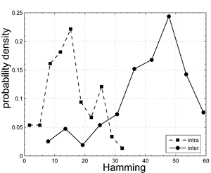
Intra image matching
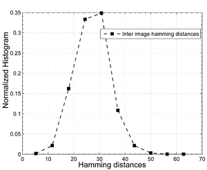
If we look at the resulting Hamming distances when we match the binarized projected descriptors from a query image against all descriptors from an image repository, we get the left figure. The expected Hamming distance is 30. As this is lower than the average Hamming distance between binarized projected descriptors from identical but distorted images the Hamming distance can not be used solely in this dataset to identify distorted images. Deployment of a simple heuristic that samples points for geometric consistency enhances the situation considerably.
Example usage
Download
Paper
M. Diephuis, S. Voloshynovskiy, O. Koval, and F. Beekhof, "Statistical Analysis of Binarized SIFT Descriptors," in Proc. 7th International Symposium on Image and Signal Processing and Analysis, Dubrovnik, Croatia, September 4-6, 2011. [pdf|bib], [Presentation]
Matlab Code
Dependencies
The code uses the following libraries:
- VLFEAT by Andrea Vedaldi and Brian Fulkerson
- XML_IO_tools by Jaroslaw Tuszynski
References and Dependencies
Please site as:
@inproceedings { DiephuisSeptember4-62011,
author = { M. Diephuis and S. Voloshynovskiy and O. Koval and F. Beekhof },
title = { Statistical Analysis of Binarized SIFT Descriptors },
booktitle = { 7th International Symposium on Image and Signal Processing and Analysis },
year = { September 4-6, 2011 },
address = { Dubrovnik, Croatia },
timestamp = { 2011.07.28 }
}
